Application of freely available software packages and Machine Learning methods for processing large arrays of mass spectrometric data for non-target analysis of beer samples by gas chromatography-mass spectrometry

Introduction

Mass spectrometry is believed to be the most sensitive, selective, and highly informative method for organic compounds identification and quantification. Ability to obtain comprehensive information on hundreds of compounds in a single GC-MS run, including their structural information, fragmentation patterns make it a powerful tool for non-targeted research.

Non-targeted research methods include the task of detecting molecules that allow distinguishing groups or classes of samples by isolating biomarkers from large arrays of mass-spectrometric data [1-3]. Thus, non-targeted research approaches are inherently more holistic, compared to the methods of targeted analysis. Non-target analysis approaches are more based on hypotheses, since they do not rely on a predetermined known set of compounds, as in the case of target analysis, but take into account all detected signals.

The non-targeted analyses methods are often used in areas of food sciences, environmental studies, and forensic examination, as well as in systems biology and metabolomics research. Metabolomics is a typical example of non-targeted analysis application, especially when a comprehensive study of unique chemical “fingerprints” specific to various metabolic processes occurring in living cells is required [4].

Application of non-target analysis methods became possible due to wealth of information obtained from mass-spectrometric data, allowing to implement many approaches to its interpretation, including, in particular, machine learning for clustering and effective recognition of patterns of mass-spectrometric signals.

There are several pre-requisites for non-targeted analysis, to begin with the choice of separation method and scanning mode of the analyzed samples. However, no uniformity of the separation method warrants precise similarity of the data, such as, for example, identity of the elution time of peaks presents in all the studied samples (common peaks), which subsequently requires additional steps of automatic signal identification followed by selection of algorithms for alignment their time characteristics and grouping. Important steps of non-target analysis are a visual representation of the features clustering, validation, and identification of markers for each cluster.

Gas chromatography in combination with various methods of mass spectrometric detection (GC-Q/GC-TOF) provides the most extensive amount of information about the chemical composition of the sample, therefore it is considered the «gold standard» for the analysis of compounds in non-target analysis studies [5]. An important feature of the non-target analysis based on using the GC-MS method is the ability to effectively identify compounds due to the use of electron ionization sources for the fragmentation of vaporized compounds coming from the chromatograph. The fragmentation spectra of compounds obtained during electron ionization are specific, stable, and highly informative. This fact stimulated development of appropriate mass spectrometric libraries for compound identification by GC- MS. And today, such libraries contain spectra for several hundred thousand low-molecular compounds from various fields of science (libraries of NIST, Wiley, GMD, etc.) [6-9].

To date, many software tools have been created for processing chromatography mass spectrometric data. Such tools can most often be divided into two categories: (a) commercial software that is provided by manufacturers of mass spectrometric equipment; (b) freely available software packages developed by various independent groups of scientists or enthusiasts. Examples of commercial products include the following software packages: MassLynx (Waters Corporation, Milford, Massachusetts, USA), ChromaTOF (LECO Corporation, St. Joseph, Michigan, USA), ChemStation (Agilent Technologies, Santa Clara, California, USA), AnalyzerPro (SpectralWorks, Runcorn, UK), ClearView (Marks International, Ronta, Kinon, Taf, UK) and IonSignature (Ion Signature Technology, North Smithfield, Rhode Island, USA). Such packages are typically designed for ease of use. The calculation modules of such software packages are running hidden behind their friendly graphical user interface (GUI). Most of the software packages are supplied as an integral part of instrument bundle, to ensure their wide distribution among the scientific and research community [10]. On the downside, they are designed to only work with specific data file formats provided by relevant instrument manufacturers, impeding further multi-format analysis of data from devices of various manufacturers.

Recently, a number of freely available software packages for processing large arrays of mass spectrometric data have been developed and put into use. The software if this kind is becoming increasingly available with open source and a “free” license. [11-15] Notably, the source code of such programs is available for viewing, studying and changing, in order to have control over the data processing algorithms performed, change or test new calculation structures, introduce new methods, and also change the ways of displaying the results [10]. The interfaces of such software packages typically read open data formats (*.xml, *.mxml and *.netCDF) and thus don’t depend on specific manufacturer’s format.

Until recently, very popular freely available standalone software package for processing GC-MS data has been AMDIS tool (NIST, USA) [20]. These days community of scientists has proposed several software platforms for processing and analyzing mass spectrometric data – SpectConnect [18], MetaboAnalyst [16, 17], XCMS-online [11] and Metabolome Express [19]. They work through any web browser interface and can be accessed by every researcher. The advantage of such platforms is full access to data processing functions [10]. In particular, the SpectConnect platform is aimed at detecting various biomarkers [20] in metabolomic studies and can use a list of suspected components (biomarkers) previously extracted in AMDIS [20]. The MetaboAnalyst platform provides a full cycle for high-performance metabolic research [16, 17] from processing initial data to statistical analysis, while it employs another popular platform for preprocessing data – XCMS [11]. Cloud version of the XCMS platform (https://xcmsonline.scripps.edu/) today is the most popular online platform for preprocessing mass spectrometric data and various statistical calculations [11]. An interesting fact is that XCMS platform [23] turned out to be the second most widely used an open-source tool for analysis of chromatography-mass spectrometric data as per the Journal of the Metabolomics Society [21] annual review, despite the fact that it was primarily developed for HPLC-MS data analysis and was not originally intended for GC-MS data [22].

Beyond the cloud version of the platform, XCMS permits use freely available an open-source algorithm package [23] in various software environments, such as R (http://www.r-project.org/) and Python (https://www.python.org/) [24-26] for filtering data, detecting peaks (“matchedFilter” and “centWave” algorithms), comparing, correcting their retention times (“PeakGroups” and “Obiwrap” algorithms), as well as grouping the selected signals into structures [27, 23]. Such algorithms and methods operate a large number of parameters to be optimized for the correct choice of the parameters, crucial for the successful application and study of non-target analysis data. Notably, this is not an easy task, since the choice of some parameters is not intuitive, especially if the process underlying the algorithms is not fully understood. Besides, analytical specifications of the instrument used for data acquisition affecting results require deep knowledge in of mass spectrometry and chromatography [26, 28].

There are simple approaches to processing GC-MS data, including using only algorithms for data alignment according to so-called list of previously detected compounds signals. The list of previously detected compounds, either by commercial manufacturer’s software based on peak shape and its signal to chemical noise ratio, or by AMDIS data deconvolution program [20] is fed directly to such algorithms. A similar list of peaks should be created for each chromatogram and contain the measured compound peak areas along with their retention times on TIC. An example of such algorithms is the GCAlignR software package [29].

The purpose of this article is to compare two approaches of non-target analysis for commercial beer sample data by freely available software packages for processing large arrays of mass spectrometric data in order to demonstrate working algorithms and optimization parameters for clustering data according to the composition of their volatile and semi-volatile fractions. The algorithms for preliminary data processing, normalization with subsequent data interpretation based on graph algorithms (hierarchical, non-hierarchical clustering and PCA) are considered.

2. Materials and methods

88 samples of canned beer (dark and light varieties of ale, lager, stout) bought in local supermarkets were used as objects of research. All reagents used in the study were classified as High-Quality Grade, or HPLC grade.

1000 µl of beer was added to a pre-conditioned autosampler vial containing from 50 to 300 mg of anhydrous magnesium sulfate, then placed on a shaker for 10-15 seconds. Next, 500 µl of ethyl acetate was added and mixed on an orbital shaker at 220 rpm for 10 minutes. Then the mixture was centrifuged at 3500 rpm for 5 minutes, and 1.0 µl of supernatant layer was injected into GC-MS system. The sampling was carried out by an automatic injector at a height of 23 mm from the bottom of the vial, to ensure only the upper layer fraction of the mixture was injected into the GC inlet.

The Q-Tek GC-MS was chosen as a research tool. The operating modes and parameters of the instrumental method are presented in paragraph 2.1.

Preliminary processing and preparation for data export, as well as automatic integration of the obtained chromatograms were performed with proprietary GC-MS software (Q-Tek, Montenegro).

 

2.1. Data acquisition parameters

GC separation parameters:

GC Column:	Rtx-5MS (30 m x 0,25 mm; 250 µm)
Carrier gas type and flow, mode:	(He) 1,0 mL/min, constant flow
Injection volume:	1 µL, sampling depth 23 mm from bottom of a vial
Inlet temperature and split ratio:	Split mode 50:1, t=200°C
Oven t° program:	50°C hold 1,0 min; 20.0°C/min to 200°C, hold 1,5 min.

Mass spectrometric detector:

Ionization mode:	Electron Impact at 70 eV
Ion source temperature:	230°C
Transfer line temperature:	250°C
Scan range:	SCAN (50 – 250 Da)
Scan rate:	10 scans/sec

The obtained chromatograms for three beer samples are shown in Figures 1-3:

Fig. 1. Chromatogram of the dark Ale beer extract

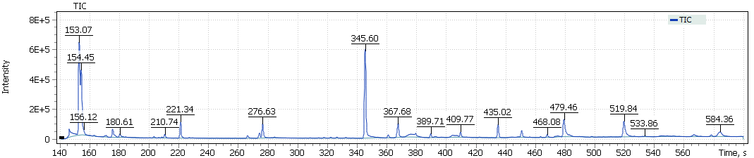
Fig. 2. Chromatogram of the light Lager beer extract

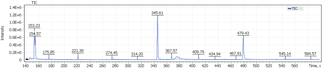
Fig. 3. Chromatogram of the IPA extract

In this study two approaches of the data post-processing were tested and implemented, in order to prepare data for further clustering of available beer samples, as well as to identify specific markers for each cluster within the framework of non-targeted analysis.

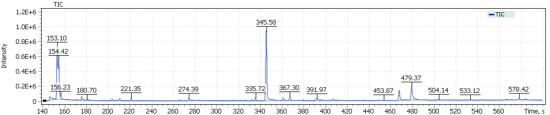
1^st approach. Using the integral values of the total ion current chromatogram (TIC) signals to convert them into tabular values (lists) for subsequent profiling and comparison. 

Fig.4. The scheme of the approach using integrated TIC signals and GCAlignR algorithm

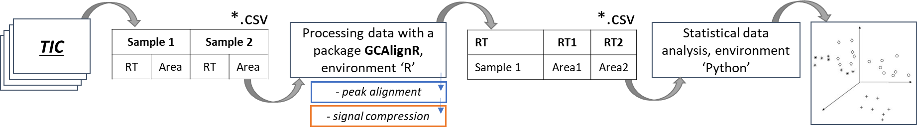
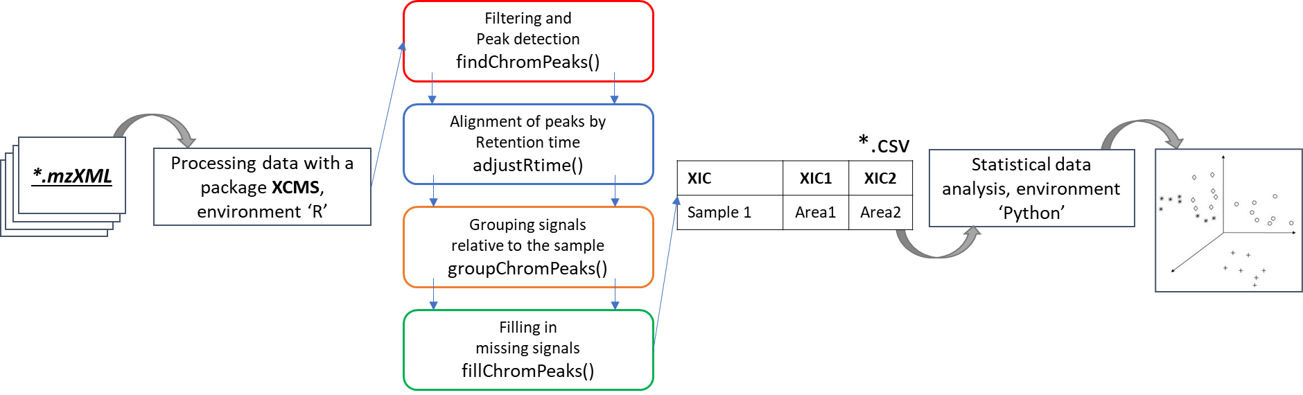
2^nd approach. Using the integrated extracted ion chromatogram (XIC) signals for selected characteristic ions to specific sample components. To follow convert them into tabular values (lists), profiling, and comparison.

Fig. 5. The scheme of the approach using integrated XIC signals and XCMS algorithm

For comparison of the two above approaches, it was proposed to use results of machine learning methods (namely, support vector machine (SVM) and stochastic gradient boosting (SGB)) to build a table of error matrix and calculate the average accuracy of data clusterization.

2.2. Theory and application of non-target analysis methods (preliminary data preparation).

Preliminary data preparation was performed in the R computing environment, designed specifically for mathematical modeling and graphical representation of data. R can be used as a simple tool to edit data tables, to do statistical analyses (for example, t-test, ANOVA or Regression analysis), as well as for more complex long-term calculations, in particular, to test hypotheses, to build vector graphs and maps. The R environment is a freeware and can be installed on both Windows and UNIX-class operating systems (Linux and macOS X).

The difference between mass spectrometric data and classical gas chromatography data is availability of a mass spectrum, that significantly increases specificity of the method. The mass spectral characteristic of the signal on TIC chromatogram is a set of mass peaks related to the fragmentation of molecules in the scanned mass range. In this case, each mass peak of the spectrum can be restored (reconstructed) as a separate mass signal (for example, EIC chromatogram). Therefore, for a comparative analysis of various beer samples using a GC-MS system two different approaches to analysis can be used, namely: comparison of total ion current (TIC) signals and comparison of reconstructed mass peak (XIC) signals.

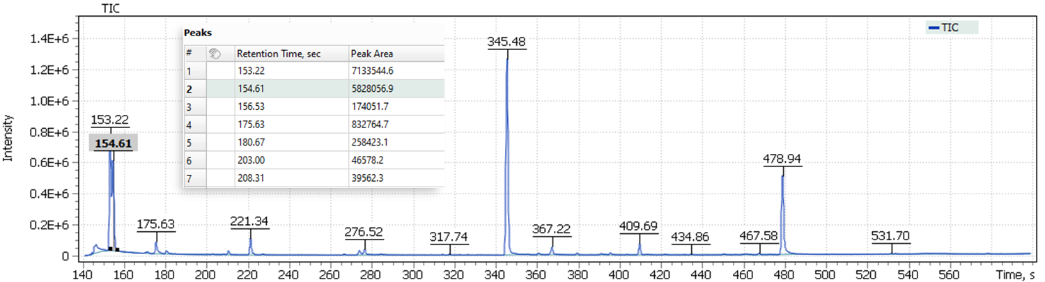
The first approach to the data postprocessing, used in this article, is based on samples comparison by their chromatographic signals derived from automatically integrated TIC chromatograms by Q-Tek GC-MS Software. The automatic integration procedure involves detection of components present in the sample and formation of a table of their characteristics (Retention Time (RT) and Signal integral (Area)) (fig. 6).

Fig. 6. Example of a table of characteristics signals on a TIC chromatogram

Compound retention times in similar samples are well known to drift back and forth over long series of repeated chromatographic experiments. The reasons for this phenomenon have to deal with laboratory environmental conditions, precision of gas flow controller, column resource, sample loading, as well as possible chemical interactions between various components of the analyzed mixture during the experiment. Therefore, the retention time alignment of chromatographic peaks corresponding to the same component in different samples is a critical step for the next data processing step.

To perform peak alignment, the GCAlignR data post-processing algorithm was used in this work, which was originally created as a tool for alignment the retention time of peaks obtained after flame ionization detection, but almost immediately the algorithm became popular for mass spectrometric signals too. The GCAlignR algorithm is based on dynamic programming [30], which includes three consecutive steps for data alignment, followed by a step for comparing peaks belonging to presumably homologous substances in different samples.

The first alingnment step is adjustment of systematic linear shifts between integrated peaks and the reference sample to account for systematic retention time shifts between the samples. Such a step is often referred to in literature as “full alignment” [31]. As a reference sample – by default – the algorithm selects the sample that is most similar to all other samples, on average.

On the second step, individual peaks in all samples are aligned by sequentially comparing retention time values of the peaks of each sample with respective average values of all previous samples. In the literature, such step is often referred to as “partial alignment” [31].

The third step takes into account the fact that a number of homologous peaks will be sorted into several rows, which can also be subsequently combined into one peak. All the stages of the algorithm are described in more detail in the article [32].

As shown in Figure 4, the input data format for the GCAlignR algorithm is a list of peaks, which consists of retention times and random variables (for example, peak height or peak area) that characterize each peak in the data set, respectively. The approach implemented in this article is based exclusively on peak retention times and their areas, so the quality of peak alignment strongly depends on the initial quality of data acquisition and peak detection parameters used. Simply put, the sharper the peaks extracted from the chromatographic profiles, the better the peak alignment result will be.

The GCAlignR algorithm output is a table of aligned peaks in the chromatogram profile relative to all analyzed samples.

> aligned_peak_data

> In total 75 substances were identified among all samples. 4 substances were present in just one single sample and were removed. 71 substances are retained after all filtering steps.

> For further details type:

>  ‘gc_heatmap(x)’ to retrieve heatmaps

> ‘plot(x)’ to retrieve further diagnostic plots

Having the algorithm applied, 75 peaks were detected, 4 of which were present only in single samples, and such peaks were excluded from the total set of peaks. Thus, 71 peaks were accepted for further analysis after data filtering and alignment.

Fig. 7. Table of deviations from the detected components average retention time

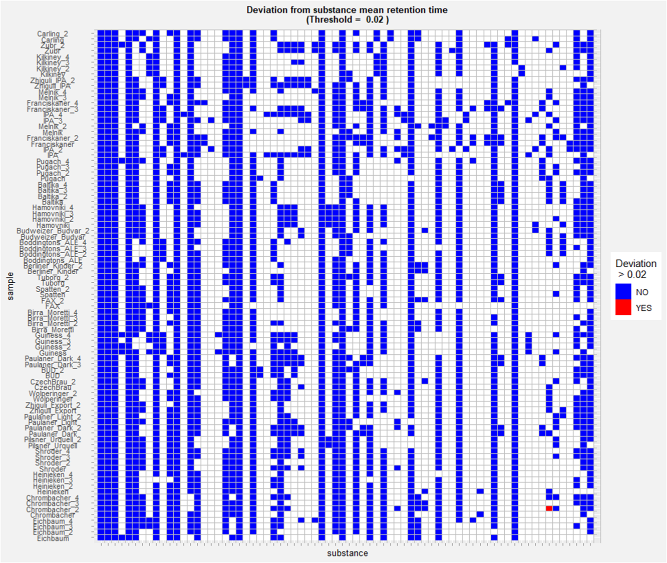
Fig. 8. Diagram for the number of detected peaks corresponding to each beer sample, a result of GCAlignR alignment

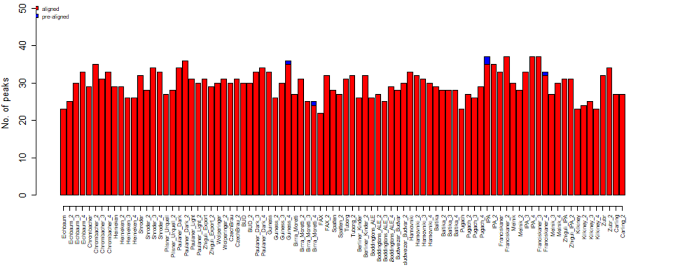
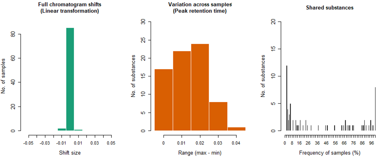
Fig. 9. Diagrams of GCAlginR algorithm results

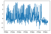
The second approach to data post-processing is based on comparing the extracted mass peaks at each recorded point on the TIC chromatogram. In short, GC-MS data can be represented as a time series of scans of the mass spectrum (Fig. 10), where each scan consists of a series of pairs (mass (m/z) – intensity). Thus, it becomes possible to convert raw data into a two-dimensional matrix [10] ([m/z] [intensity at each point of the scan time on the chromatogram]).

The freely available software package for processing large arrays of mass spectrometric data XCMS includes many methods of working with such two-dimensional matrices, including convertation of the entire array of mass spectrometric data (of all samples) into required format.

The raw data is imported using the “readMSData” method (Fig. 11):

>> MS level(s): 1

>> Number of spectra: 365997

>> MSn retention times: 2:21 – 9:60 minutes

The “findChromPeaks” function of the XCMS package helps to derive probable signals of mass peaks relative to their chromatographic retention time axis from the loaded data array. Notably, two algorithms for detecting mass peaks are available to the function: Matched Filter Param, as well as CentWaveParam, which was used in this work. The CentWaveParam algorithm performs mass peak detection based on a Continuous Wavelet Transform (CWT), which can detect close and partially overlapping signals with different base widths (retention time) [33].

Fig. 10. Conversion of GC-MS data into time series of mass spectrum scans

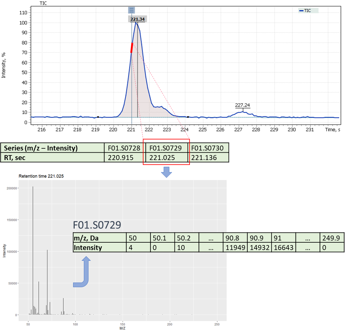
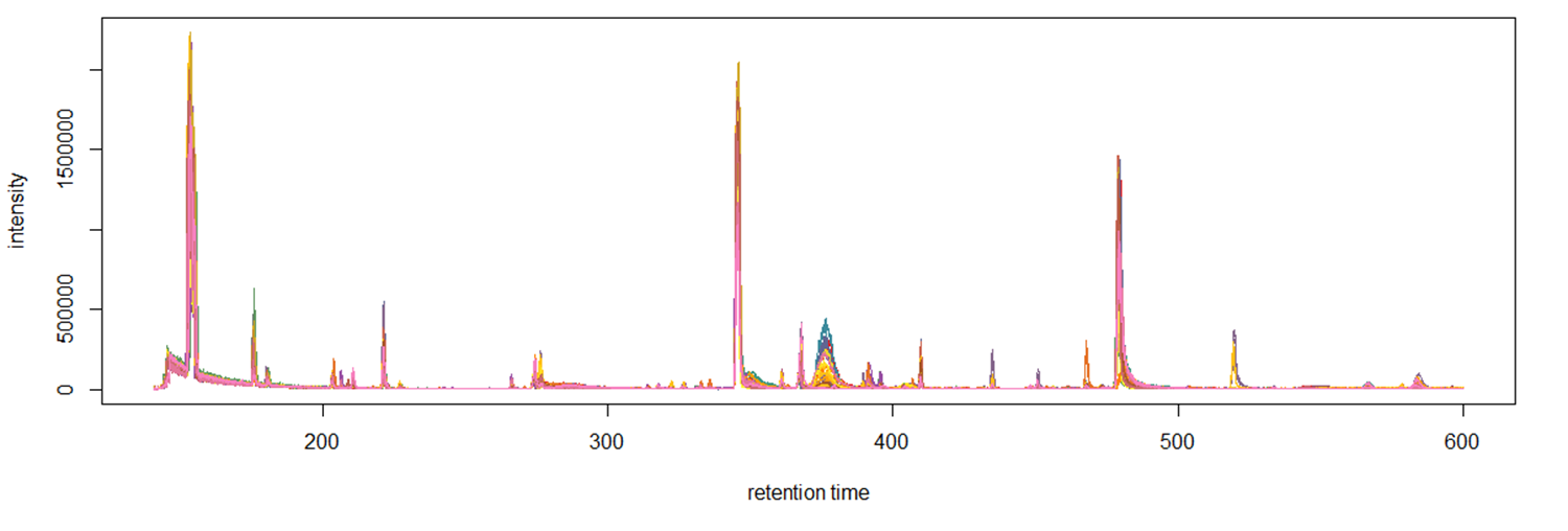
Fig. 11. Base Peaks Cromatogramm (BPC), opened in the R computing environment by readMSData method

The CentWaveParam algorithm can be configured with several parameters, the most important being the peak width (peakWidth) and the mass accuracy (ppm). The peak width is the value of the minimum and maximum expected width of the mass peaks (in sec), that depends on settings of the chromatographic separation method. Most often, in gas chromatographic separations, the expected width of a mass peak is from 1 to 3 seconds. The single quadrupole MS systems are considered to have accuracy of a single mass unit, therefore, in this study, the value 1000 was used. The algorithm application resulted in data presented on Fig. 12:

>> method: centWave

>> 37811 peaks identified in 88 samples.

>> On average 430 chromatographic peaks per sample

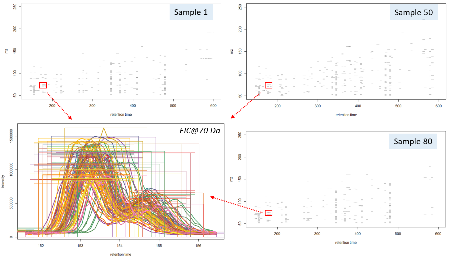
The algorithm detected 37’811 mass peaks altogether in all 88 beer samples, i.e. 430 mass peaks per sample. This amount of information on chemical composition of a sample made it possible to use Machine Learning algorithms for reliable sample clustering for non-targeted analysis, comparison, and identification of different features. The results of working CentWaveParam algorithm are shown in Figure 12, noting two closely eluting partially overlapping peaks to have been clearly separated mathematically, and a map of detected mass peaks plotted in “m/z – retention time” coordinates for three different beer samples is also presented.

Fig. 12. Results of working CentWaveParam algorithm: reliable detection of mass peaks on chromatographic profiles of three beer samples is shown.

As noted earlier, the chromatographic peaks alignment is a crucial stage of data preprocessing. The same requirements apply for the detected mass peaks array (XIC). In XCMS software tool, there are two methods for the retention time correction, namely: peakGroups [11] and Obiwarp [34]. Obiwarp alignment method was used later in this work.

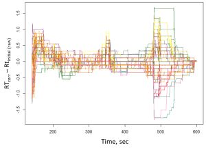
Fig. 13. The results of the Obiwarp method. (Chart in the left frame shows the difference between corrected and original retention times along the retention time axis (in sec). The plots on the right-side show signals of the mass peak at 70 Da: A – before; B – after applying the alignment method.)

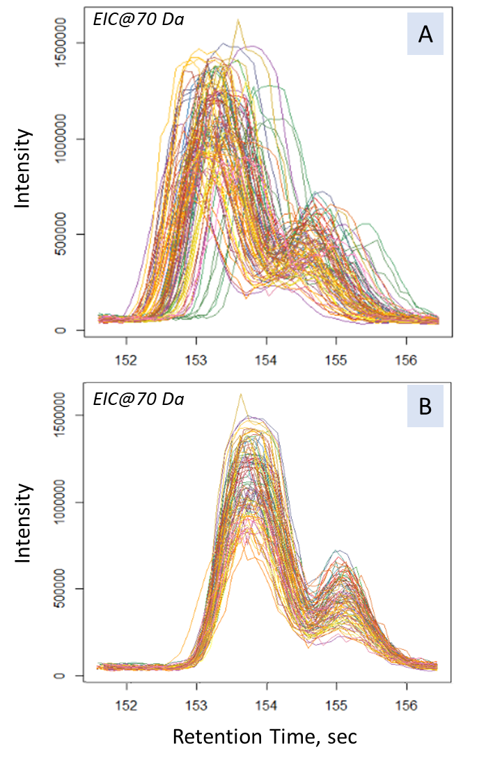The main criterium for the alignment results validation lays in evaluation of difference between the initial (raw) and corrected retention time. In our case, all the samples were analyzed within a short period of time, and the difference was less than two seconds, which is an acceptable result of the method application. An excessively large difference between the corrected and the initial retention times would indicate instability of the chromatography-mass spectrometric system or incorrectly peak alignment parameters.

The final step of post-processing for mass spectrometric data by XCMS tool is correlational analysis of the data, where mass peaks of the components are grouped into one segment to form a general interconnection and for the component signal identification. XCMS uses two methods to achieve that: peak density [11] and nearest [35].

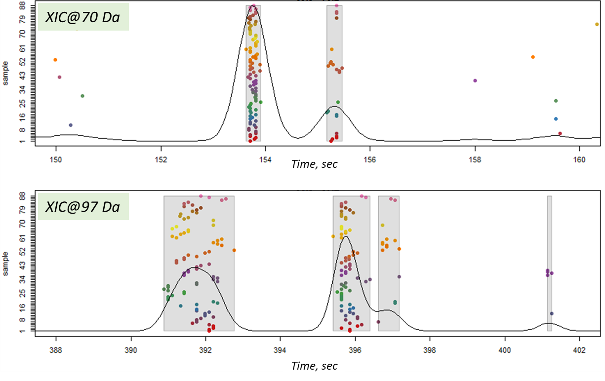
In this article, the peak density method was used, which iterates through m/z slices in the data array and groups mass peaks in each slice by features (within one or several slices) based on the mass peaks’ retention times. Thus, it is expected that the mass peaks constituting the signal of the same component will have the same retention times. And if similar mass peaks are found in many samples, then such a population will be expressed by a high density of mass peaks at the point of a component retention time. The result of the peak density method is shown in Figure 14. Notably, even close-standing mass peaks were successfully grouped into separate components of the sample profile.

Fig. 14. The result of matching mass peaks on a slice (peak density method in XCMS package).

3. Results and discussion.

The final data processing and distribution of many samples into clusters was carried out in an open-source Python computing environment. The Python language has a clear and consistent syntax, well thought-out modularity, and scalability, so that Python source code is easy to read and control. Currently, Python with the NumPy, SciPy and MatPlotLib packages is actively used as a universal environment for scientific calculations to replace for common specialized proprietary packages, say Matlab, due to their equal functionality at a lower entry threshold [36].

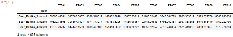
Figures 15 and 16 show tabular data (lists) prepared in R environment. The columns of the table contain the features (integrated signals) pertinent to each sample, and the sample names are the row names of the table. The list in Figure 15 has a size of 88 samples, 71 features (columns) each. The list in Figure 16 has a size of 87 samples and 638 features altogether.

Fig. 15. The features table derived by application of GCAlignR algorithm upon data from TIC chromatogram integration:

Fig. 16. The features table derived from XCMS algorithm application on data from XIC chromatogram integration

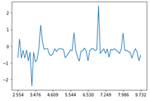
Complexity and variability of biological matrices chemical composition lead to a broad range of features and, accordingly, the features numerical spread values so there is a risk for a machine learning algorithm to automatically decide that a feature having higher spreads of values is more significant than the one where the spreads of values are lower. However, which is not the case, since all the features are significant. Therefore, the general scaling of features helps to compare unrelated objects with different measurement units and ranges after their conversion to comparable values. Therefore, methods of data scaling and standardization were applied further in this work, namely StandardScaler structure in sklearn.preprocessing library. The results of scaling for beer sample (sample #10) by the approaches 1 and 2  are shown in Figure 17.

Approach 1 (GCAlignR)	Approach 2 (XCMS)	Fig. 17. The alignment results plotted for the beer sample (#10).

3.1. Cluster analysis.

Clustering (or cluster analysis) is a task of dividing a set of objects into groups (called clusters). There should be “similar” objects inside each group, while objects of different groups should be as different as possible. The main difference between clustering and classification is that the list of groups is not clearly defined and is determined during the algorithm application.

Performing cluster analysis in general is reduced to the following stages:

1) Calculating the similarity measure values between objects and determining the optimal number of clusters.

2) Using the cluster analysis method to create groups of similar objects (clusters). Reducing dimensionality of data array, if necessary.

3) Presentation of the analysis results.

Having the clustering results obtained and reviewed, it is possible to adjust the selected metrics and clustering methods until the optimal result is achieved.

3.2. Calculating similarity measure values for the objects

Choosing optimum number of clusters is a top challenge in data clustering. The number of segments is a key parameter for several clustering algorithms, such as, for example, the k-means clustering method, agglomerative clustering, or distribution-based clustering (GMM – Gaussian mixture distribution).

The clustering process mostly involves Machine Learning without a teacher approach. There are two most common clustering methods: non-hierarchical clustering – the k-means method, used to optimize a certain target function; and hierarchical clustering (dendrogram), having the advantage over the k-means algorithm in no need for prior determination of clusters number. However, hierarchical clustering does not work well in case of big data (large amount).

The hierarchical clustering results are usually presented as a dendrogram – a tree-like clustering graph. Figures 18 and 19 show hierarchical clustering as per Ward’s rules [37].

Fig. 18. Dendrogram of hierarchical data clustering obtained with GCAlignR approach.

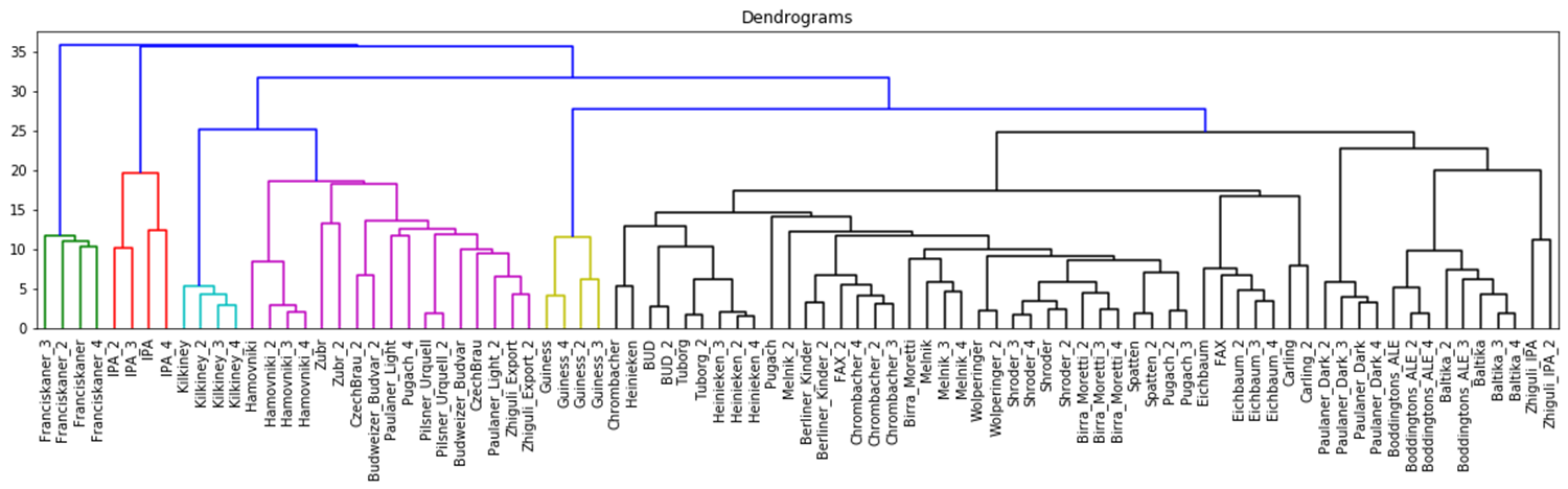
Fig. 19. Dendrogram of hierarchical data clustering obtained with XCMS approach.

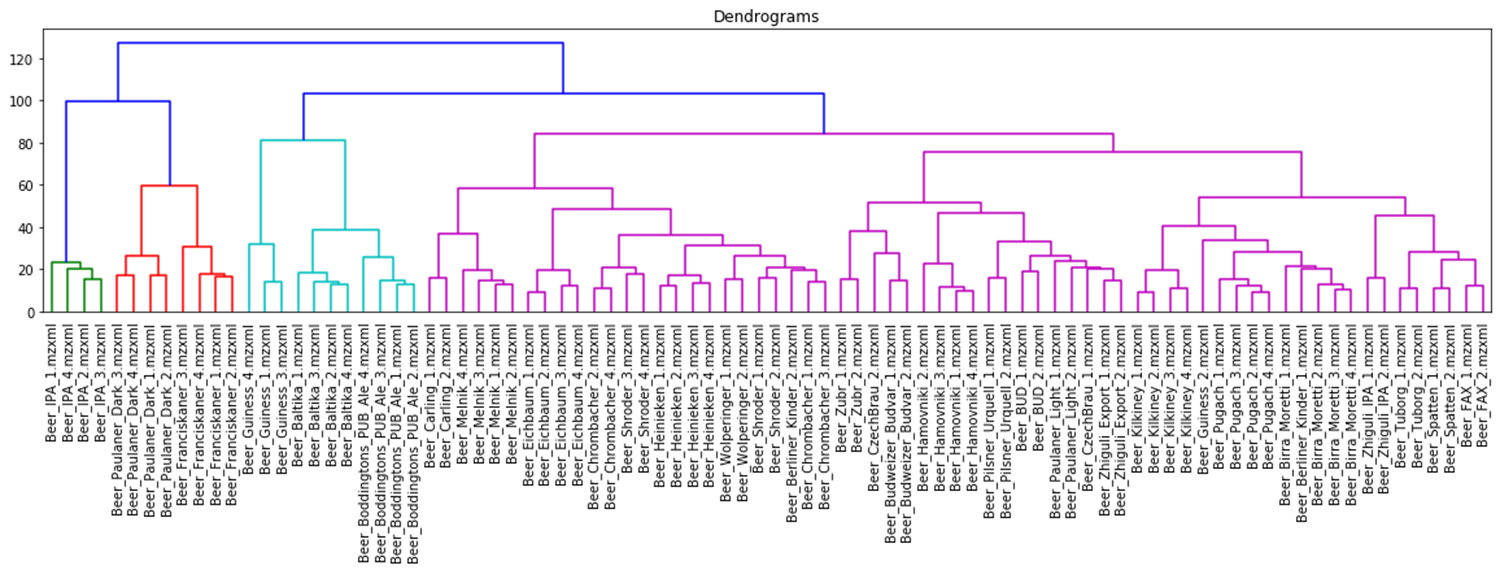
The color grouping of the dendrogram shows the data derived from TIC chromatogram integration were divided into 6 clusters, while the data from XIC chromatogram integration were divided into 4 clusters.

A quantitative measure of how faithfully a dendrogram preserves the pairwise distances between the original unmodeled data points is cophenetic correlation (more precisely, the cophenetic correlation coefficient). Although it has been most widely applied in the field of biostatistics (typically to assess cluster-based models of DNA sequences, or other taxonomic models), it can also be used in other fields of inquiry where raw data tend to occur in clusters. The cophenetic correlation coefficient determines the distance between two objects on the dendrogram and reflects the level of intra-group differences at a point when these objects were first combined into one cluster [45]. All possible pairs of such distances form a posterior distance matrix between objects based on the results of clustering. At the same time, the closer cophenetic correlation coefficient value is to 1, the better clustering preserves the original distances. The SciPy library contains a function for cophenetic correlation coefficient calculation, the results were, as follows:

Data obtained as a result of the GCAlignR algorithm	0,721	Number of clusters	6
Data obtained as a result of the XCMS algorithm	0,717	Number of clusters	4

The cophenetic correlation coefficients for both approaches appear to be comparable, the values are both near 1, therefore, data clustering with hierarchical clustering approach was successful. Quite exemplary, that Irish Guinness beer, IPA and dark beer sorts were attributed to separate groups; two large clusters populated by variety of light beer sorts are also observed.

3.3. Application of the cluster analysis method for creating clusters

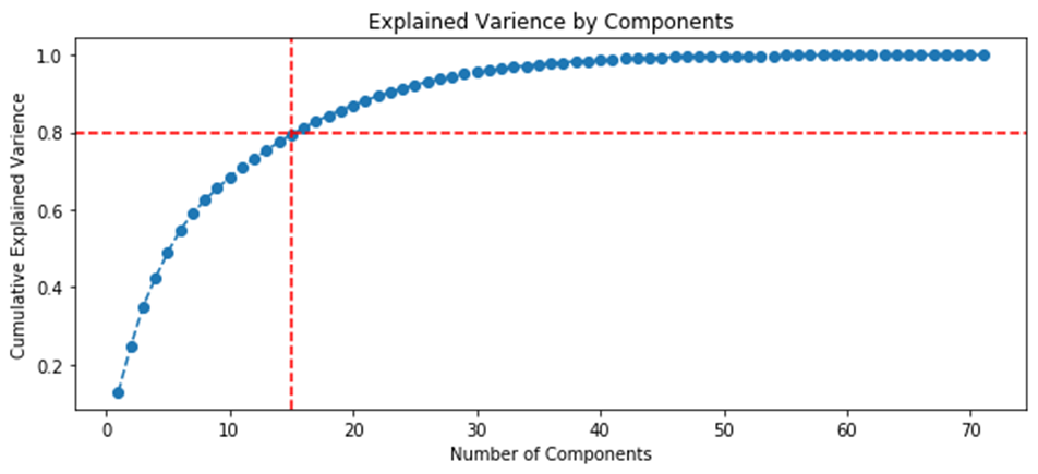
K-means clustering is simple and most popular algorithm for non-hierarchical data clustering. As a rule, the goal of the k-means algorithm is simple: to group similar data points and identify the main patterns with a fixed number of (k) clusters. For more information about the k-means algorithm, see this article [38]. To facilitate search for similar points in large data array, there is a data dimensionality reduction technique – the principal components analysis (PCA) method. The purpose of PCA method is to find linearly independent variables that can represent data without loss of important information. Thus, the method is used to replace several initial variables by converting them into a smaller number of new variables (reducing the dimension), ranking the new variables by their attributed variance parameters with the condition of losing the least amount of information. These newly introduced variables are called the principal components (PC).

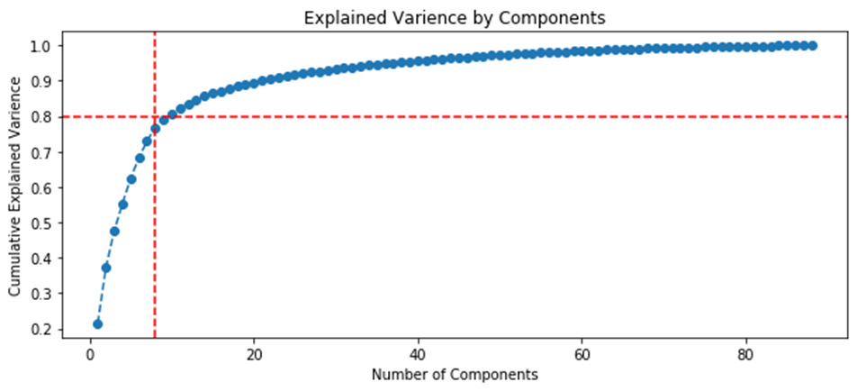
Figure 20 shows ranking of variables by variance relative to the initial data set and highlights the number of variables (components) required to explain 80% of the variations between the samplings.

Fig. 20. Graphs of the ranking of variables by variance.

Approach 1 (GCAlignR), 15 components for 80%	Approach 2 (XCMS), 8 components for 80%

At the next stage, will be done a clustering by k-means method within the selected number of variables (components). The number of clusters is most often estimated by quantitative methods for assessing the degree of clustering. We used two methods in this work: 1) Elbow Method; 2) Silhouette Coefficient [39]. The results of running these quantitative methods are shown in Figure 21.

Fig. 21. Quantitative estimation of the degree of clustering for CGAlignR and XCMS approaches. The Left frame shows clustering diagram by “elbow” method, the right frame shows clustering diagram by “silhouette” coefficient method.

approach 1 (GCAlignR)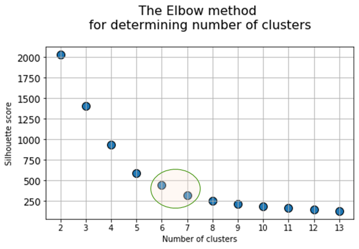
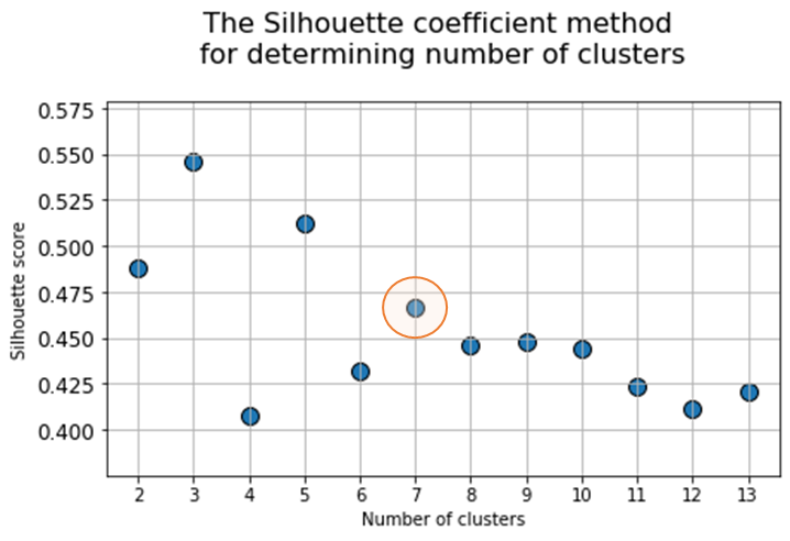approach 2 (XCMS)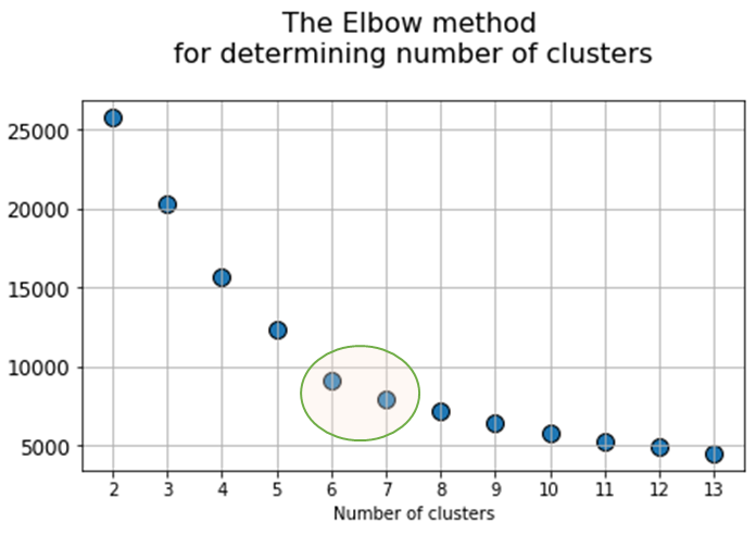

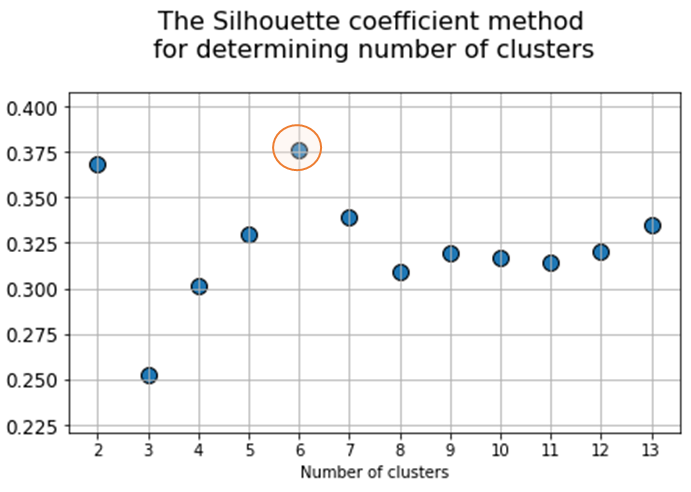From the above plots we can assume the optimal number of clusters to be 6 – 7 by “elbow” method. The main idea of the “elbow” method is that the explained variation changes quickly for a small number of clusters, and then slows down, which leads to the formation of a bend (elbow) on the curve. The bend point is the optimal number of clusters that we can use for the given data set. To validate the number of clusters, we estimated “silhouette” coefficient method, which is a calculated score for difference between the average space within a cluster and the average space to the nearest cluster for each sample normalized to the maximum value. This metric is used to calculate the goodness of a clustering technique. Its value ranges from (-1) to (1). Result «1» – means clusters are well apart from each other and clearly distinguished, while «-1» is an indication of completely incorrect clustering. Based on calculations, 7 clusters (SilCoef = 0.46) is a better choice than 6 clusters (SilCoef = 0.42) for the first approach (by GCAlignR); while 6 clusters (SilCoef = 0.375) is a good choice for the second approach (by XCMS).

3.4. Presentation of the analysis results

The final stage of the study is construction of data clustering graphs followed by data dimensionality reduction and clustering by k-means method relative to previously selected number of assumed clusters.

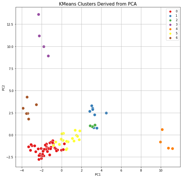
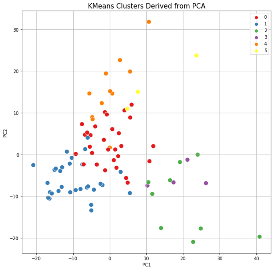
The results of clustering, as well as two-dimensional and three-dimensional graphs are presented in Figure 22. The upper graph shows the clustering for the approach based on (TIC) chromatogram integration data processed with GCAlignR method. This approach showed better distribution of samples in component space than approach 2 (using XIC).

Fig. 22. Results of data clustering in two-dimensional and three-dimensional component space.

Distribution of samples as a result of using TIC chromatogram integration data (GCAlignR)
Distribution of samples as a result of using XIC chromatogram integration data (XCMS)

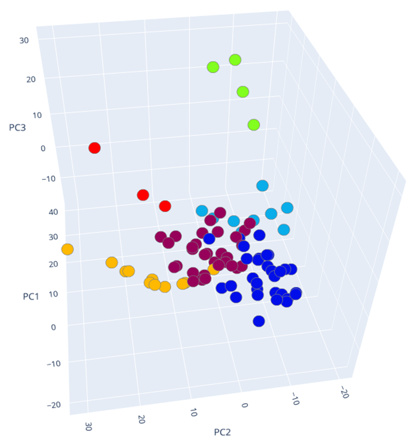The lower graph of Figure 22 shows distribution of clusters resulting from application of XCMS algorithm upon XIC chromatogram integration data. This approach is noted to result in clusters having a ribbon structure while the distribution is not as good. Finally, each beer sample gets a cluster number assigned it belongs to based on cluster analysis done.

3.5. Evaluation of the clustering quality.

To assess clustering quality, we used supervised Machine Learning that involves using a model to learn a mapping between input examples and the target variable (cluster label was used as the target variable).

About 60% of the original data set were used as training data for machine learning. The remaining 40% of the data was used to estimate the opportunity of the model (built on the training data) and, accordingly, the quality of clustering.

The following Machine Learning methods were used:

1. Support Vector Machines (SVM);
2. Stochastic Gradient Boosting (GradientBoostingClassifier, GBC).

As a result of the machine learning opportunity estimation and, respectively, the quality of clustering, the error matrix table was used, to characterize the classification by four possible outcomes:

• TP (True Positive).
• TN (True Negative).
• FP (False Positive).
• FN (False Negative).

The example of error matrix table is shown in Figure 23, where y’-axis is response of the model on the validation data set, and y – axis is the true value of the class, according to preliminary clustering.

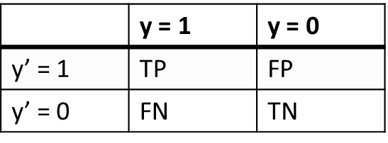
Рис. 23. Example of error matrix table

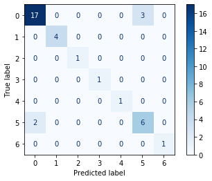
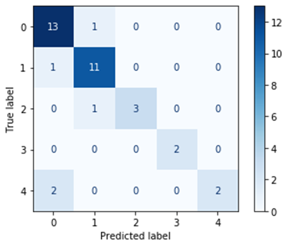
The average accuracy, measured on basis of the four outcomes by error matrix, is taken as a score of the model fit. Taking into account the fact that the data set is unbalanced, the average accuracy estimate was taken only for those clusters that had been included in the validation sample. Figure 24 shows the resulting SVM error matrix tables, for both data preparation approaches.

Fig. 24. Error matrix table for SVM algorithm.

Approach 1 (GCAlignR)	Approach 2 (XCMS)

Results of the accuracy of machine learning models and the quality of clustering:

Metrics	Approach 1 (GCAlignR)	Approach 2 (XCMS)
Average Accuracy, SVM (max 1 i.e. 100% accuracy)	0.91	0.92
Average Accuracy, GBC (max 1 i.e. 100% accuracy)	0.86	0.78

 

3.4. Interpretation of compounds identified as a result of cluster analysis.

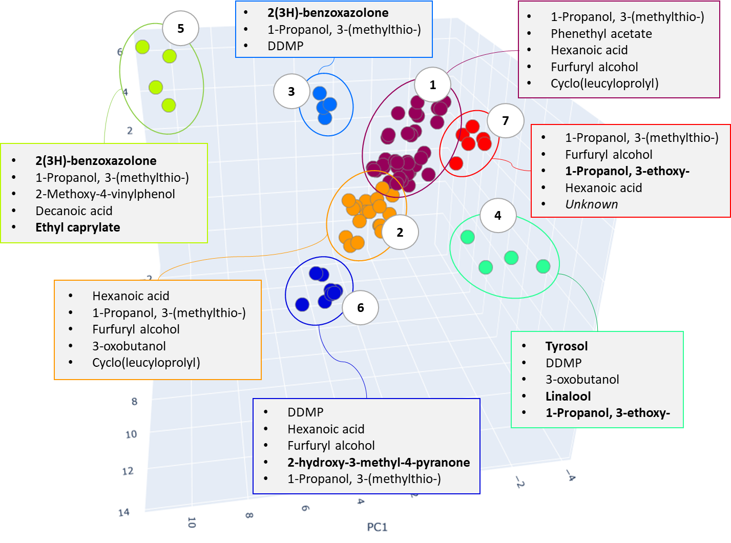
As a result of cluster analysis, compounds characterizing various beer samples were identified. In particular, Figure 25 clearly shows separation of two sorts of dark beer – Ale and Lager, attributted to clusters No. 5 and No. 3. Both clusters have main component 2(3H)-benzoxazolone, which is a specific marker of beer made from wheat malt [40], but in cluster No. 5, the ethylcaprilate component is distinguished as a characteristic marker, which is refered to in literature as contributing to specific aroma described as a fruit, floral, banana, pineapple or even cognac tint [41] in beer.

Fig. 25. The result of cluster analysis for a data set from application of GCAlignR algorithm upon TIC chromatogram integration data.

A similar result for dark beer range was revealed by the second approach of non-target sample analysis (XIC), except the both types of dark beer have been combined by the algorithm into one cluster (#3), characterized by high content of 2(3H)-benzoxazolone component.

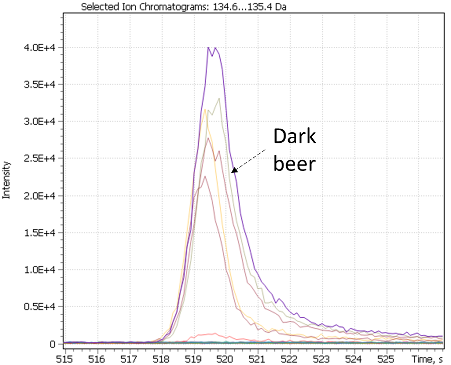
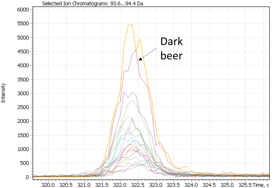
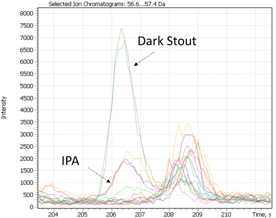
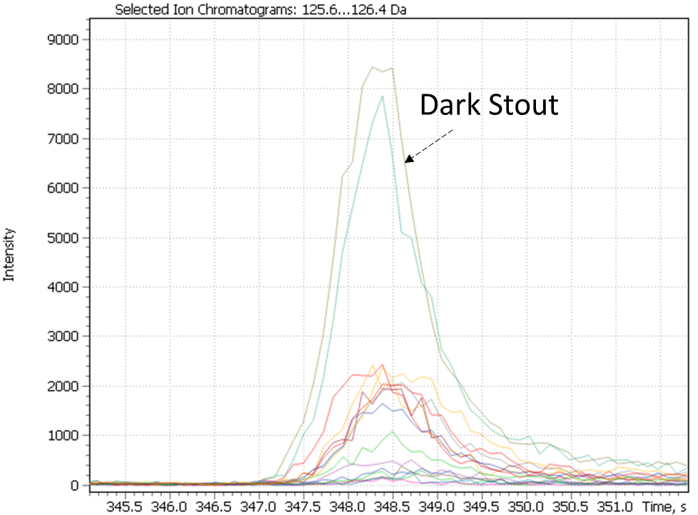
Notably, non-targeted analysis of the eXtracted Ion Current traces made it possible to detect several complementary minor markers characterizing the dark beer cluster, in particular 2-acetylpyrrol and 2-Methoxy-4-vinylphenol, as shown in Figure 26.

Fig. 26. Major and minor markers of dark beer (Ale and Lager)

2(3H)- benzoxazolone	2-acetylpyrrol	2-Methoxy-4-vinylphenol

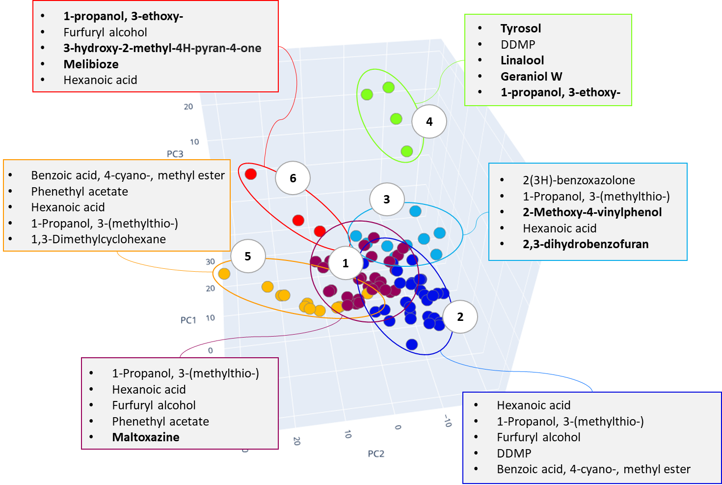
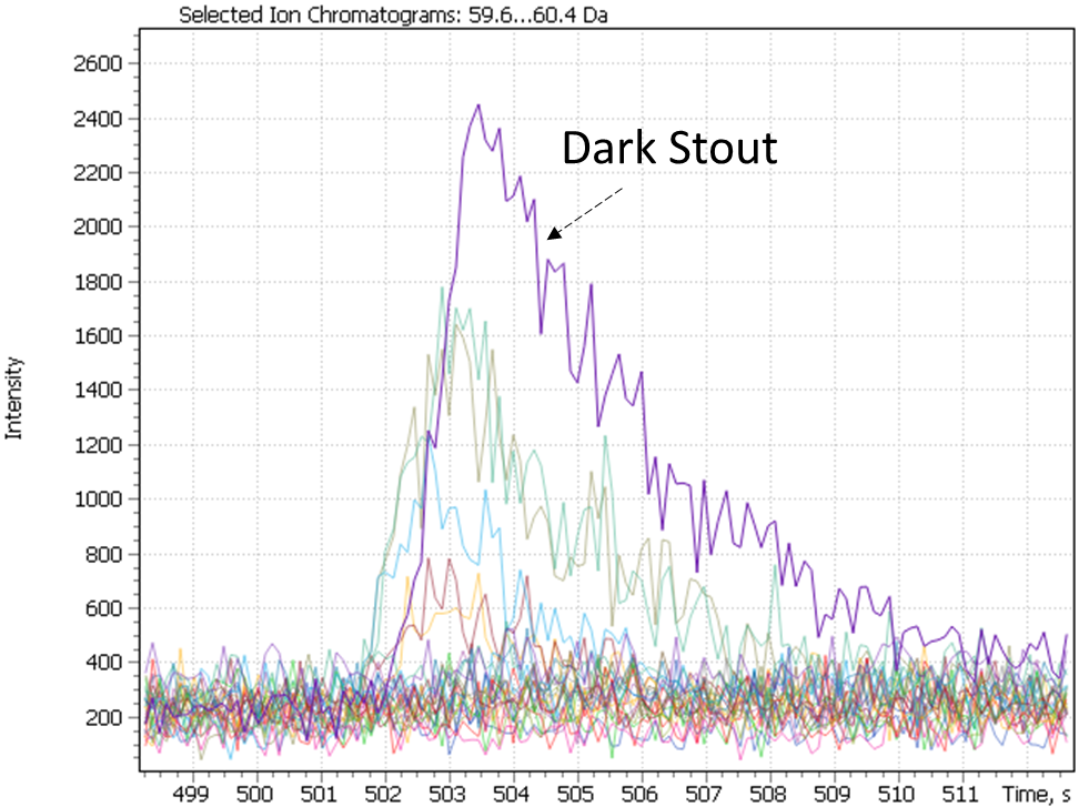
Cluster #4 in both distributions combines craft beer-IPA, characterized by a “fruit-citrus” taste due to a combination of non-standard hops. The most characteristic compounds of this cluster are tyrosol and linalool, the latter being terpene alcohol is a component important for brewers looking for intense fruit flavors in IPA. While terpene alcohols are present in hops on low level, they remain in beer throughout the entire brewing process and are less volatile than terpene hydrocarbons [42]. Another minor marker isolated on the chromatographic profiles of IPA beer is geraniol, a flavoring component yielding a floral smell present in hops. The XIC chromatogram plotted for the structurally characteristic of geraniol ion is shown in Figure 27.

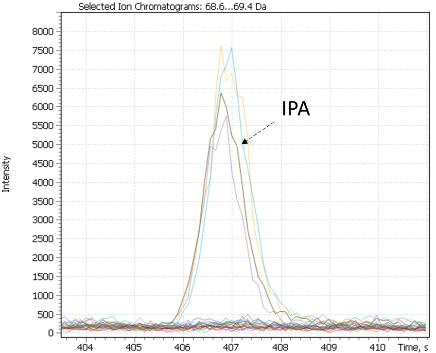
Fig. 27. XIC chromatogram plotted for geraniol selected ion (@67Da)

The clustering algorithm distributed range of light beers, into clusters #1, #2 and #6, Figure 25 shows only range of light beers of both domestic and imported origin. In most cases, specific compounds in these clusters are the same, variations are found in levels of their content, used by algorithm as basis to have these beer samples divided. In particular, beer samples with high content of several compounds were included in cluster #1, namely: phenethyl acetate, an aromatic component responsible for rose or honey aromas in beer; furfuryl alcohol, as a product of 2-furfural reduction during yeast fermentation, gives the smell of fresh bread or caramel flavor, as well as diketopiperazine. As per literary sources, the presence of diketopiperazine in beer is tolerable but its role and influence on the taste and aromatic properties of beer is still discussed by experts [43].

Cluster #2 (Fig. 25) is characterized by the presence of hexanoic acid, a likely result of the yeast metabolic activity. Its high content in beer is undesirable as causing a sharp cheese flavor and having a negative effect on the foam and taste of the drink. To avoid this, brewers often remove the yeast immediately upon the end of fermentation [41].

Fig. 28. The result of cluster analysis for data set from application XCMS algorithm on XIC chromatogram integration data.

In Figure 28, some light beer samples are besides divided into three clusters: #1, #2 and #5. It is worth noting the similarity of the isolated compounds for both research approaches used in this work. The differences related only to their individual content levels in each cluster.

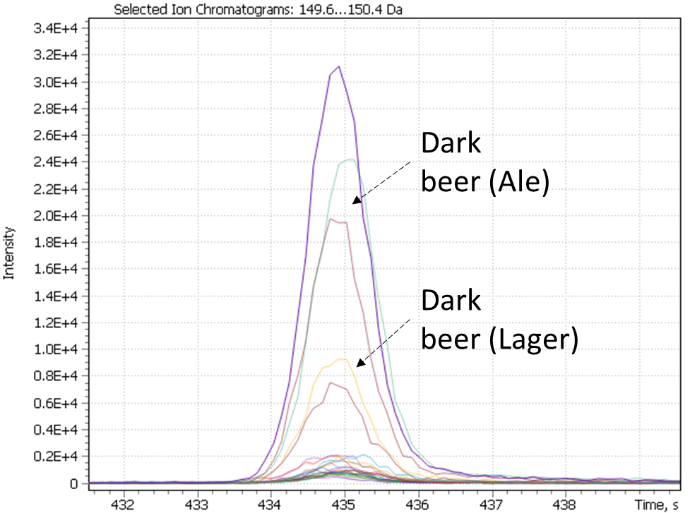
The dark stout (Ale) range was allocated to a separate cluster by both study approaches. The dark stouts (Ale) are in the cluster #7 in Figure 25, and in the cluster #6 in Figure 28. This type of beer is distinguished by the presence specific markers such as 3-ethoxy-1-propanol a metabolite of yeast; 3-hydroxy-2-methyl-4H-piran-4-one (maltol), coming from dark roasted malt grains and giving the beer a caramel taste and aroma, as well as disaccharide – melibiose. The latter, as per the literature, is one criterion used to attribute a beer to either Ale or Lager sort. In particular, whereas camp yeast is able to produce extracellular enzyme melibiose (alpha-galactosidase), serving as a catalyst for cleavage of melibiose into galactose and glucose, the Ale yeast is not able to produce such an enzyme [44].

Fig. 29. Major and minor markers of dark stout beer (Ale).

3-ethoxy-1-propanol	Maltol	Melibiose

4. Conclusions.

Two non-targeted analysis approaches have been compared to process with large arrays of raw data acquired with Q-Tek single quadrupole GCMS for a broad range of beer samples, which then exported and processed in R and Python environment by popular freeware packages GCAlignR and XCMS. In the current work, algorithms for data pre-processing and normalization were used followed by subsequent data interpretation based on hierarchical, non-hierarchical clustering, PCA and visualization tools.

Both approaches resulted in models having similar prediction quality for sample clustering, and the selected groups of markers made it possible to reliably differentiate between the types of beer. The work describes a step-by-step roadmap for data processing, that can be used for clustering food, beverage and plant extracts, not to say about other samples of biological origin used in metabolomics and lipidomics research where the task of object clustering is often required.

Q-Tek GCMS software offered an easy and seamless export of raw data array in a format readable by popular freeware tools for further statistical processing, generalization, and merge with other results on a bigger scale.

The article explores Supervised and Unsupervised Machine Learning approaches for clustering samples based on chemical compounds automatically detected in the sample profiles by Q-Tek Single Quadrupole GCMS. The developed approach demonstrated a fairly high accuracy of clustering of the studied beer samples and provided solid insights on discrimination markers.

Literary References

1. Yi, N. Dong, Y. Yun, B. Deng, D. Ren, S. Liu, Y. Liang, Chemometric methods in data processing of mass spectrometry-based metabolomics: a review, Anal. Chim. Acta 914 (2016) 17e34.
2. Boccard, J.-L. Veuthey, S. Rudaz, Knowledge discovery in metabolomics: an overview of MS data handling, J. Separ. Sci. 33 (2010) 290e304.
3. Goodacre, S. Vaidyanathan, W.B. Dunn, G.G. Harrigan, D.B. Kell, Metabolomics by numbers: acquiring and understanding global metabolite data, Trends Biotechnol. 22 (2004) 245e252.
4. Bennett Daviss, Growing pains for metabolomics // The Scientist. — 2005. — April (т. 19, № 8). — С. 25—28.
5. Mike Li, X. Rosalind Wang, Peak Alignment of Gas Chromatography-Mass Spectrometry Data with Deep Learning.
6. https://www.nist.gov/
7. https://www.wiley.com/
8. http://gmd.mpimp-golm.mpg.de/
9. Лохов П.Г. Метаболом плазмы крови для диагностики риска возникновения рака простаты, рака лёгкого и сахарного диабета 2-го типа. Диссертация на соискание учёной степени доктора биологических наук. — М., 2015.
10. O‘Callaghan et al. PyMS: a Python toolkit for processing of gas chromatography-mass spectrometry (GC-MS) data. Application and comparative study of selected tools. BMC Bioinformatics 2012, 13:115.
11. Smith CA, Want EJ, O’Maille G, Abagyan R, Siuzdak G: XCMS: processing mass spectrometry data for metabolite profiling using nonlinear peak alignment, matching, and identification. Anal Chem 2006, 78(3):779–787.
12. Katajamaa M, Miettinen J, Oresic M: MZmine: toolbox for processing and visualization of mass spectrometry based molecular profile data. Bioinformatics 2006, 22(5):634–636.
13. Bunk B, Kucklick M, Jonas R, Munch R, Schobert M, Jahn D, Hiller K: MetaQuant: a tool for the automatic quantification of GC/MS-based metabolome data. Bioinformatics 2006, 22(23):2962–2965.
14. Hiller K, Hangebrauk J, Jager C, Spura J, Schreiber K, Schomburg D: MetaboliteDetector: comprehensive analysis tool for targeted and nontargeted GC/MS based metabolome analysis. Anal Chem 2009, 81(9):3429–3439.
15. Wenig P, Odermatt J: OpenChrom: a cross-platform open-source software for the mass spectrometric analysis of chromatographic data. BMC Bioinforma 2010, 11:405–413.
16. Xia J, Wishart DS: Web-based inference of biological patterns, functions, and pathways from metabolomic data using MetaboAnalyst. Nat Protoc 2011, 6(6):743–760.
17. Xia J, Wishart DS: Metabolomic data processing, analysis, and interpretation using MetaboAnalyst. Curr Protoc Bioinformatics 2011, Chapter 14: Unit 14 10.
18. Styczynski MP, Moxley JF, Tong LV, Walther JL, Jensen KL, Stephanopoulos GN: Systematic identification of conserved metabolites in GC/MS data for metabolomics and biomarker discovery. Anal Chem 2007, 79(3):966–973.
19. Carroll AJ, Badger MR, Harvey Millar A: The Metabolome Express Project: enabling web-based processing, analysis, and transparent dissemination of GC/MS metabolomics datasets. BMC Bioinforma 2010, 11:376.
20. Stein SE: An integrated method for spectrum extraction and compound identification from gas chromatography/mass spectrometry data. J Am Soc Mass Spectrom 1999, 10(8):770–781.
21. Weber, R. J. M., Lawson, T. N., Salek, R. M., Ebbels, T. M. D., Glen, R. C., Goodacre, R., et al. (2016). Computational tools and workflows in metabolomics: An international survey highlights the opportunity for harmonisation through Galaxy. Metabolomics, 13(2), 12.
22. Rachel Spicer, Reza M. Salek, Pablo Moreno, Daniel Caсueto, Christoph Steinbeck, Navigating freely available software tools for metabolomics analysis, Metabolomics (2017) 13:106, DOI 10.1007/s11306-017-1242-7
23. Smith, C. A., Want, E. J., O’Maille, G., Abagyan, R., & Siuzdak, G. (2006). XCMS: processing mass spectrometry data for metabolite profiling using nonlinear peak alignment, matching, and identification. ACS Publications, 78(3), 779–787.
24. http://www.r-project.org/
25. https://www.python.org/
26. E. Albуniga et al., Optimization of XCMS parameters for LC–MS metabolomics: an assessment of automated versus manual tuning and its effect on the final results, Metabolomics (2020) 16:14 https://doi.org/10.1007/s11306-020-1636-9
27. Lazar, G., Florina, R., Socaciu, M., & Socaciu, C. (2015). Bioinformatics tools for metabolomic data processing and analysis using untargeted liquid chromatography coupled with mass spectrometry. Bulletin of University of Agricultural Sciences and Veterinary Medicine Cluj-Napoca Animal Science and Biotechnologies. https://doi.org/10.15835 /buasv mcn-asb:11536.
28. Wehrens et al. / J. Chromatogr. B 966 (2014) 109–116
29. https://cran.r-project.org/web/packages/GCalignR/index.html
30. Eddy SR. What is dynamic programming? Nature biotechnology. 2004; 22(7):909±910. https://doi.org/10.1038/nbt0704-909 PMID: 15229554
31. Bloemberg TG, Gerretzen J, Wouters HJP, Gloerich J, van Dael M, Wessels HJ, et al. Improved parametric time warping for proteomics. Chemometrics and Intelligent Laboratory Systems. 2010; 104 (1):65 ± 74.
32. Ottensmann, Meinolf, Martin A Stoffel, Hazel J Nichols, and Joseph I Hoffman. “GCalignR: An R Package for Aligning Gas-Chromatography Data for Ecological and Evolutionary Studies.” PloS One13 (6):e0198311.
33. Tautenhahn, Ralf, Christoph Böttcher, and Steffen Neumann. “Highly sensitive feature detection for high resolution LC/MS.” BMC Bioinformatics9 (1):504
34. Prince, John T, and Edward M Marcotte. “Chromatographic alignment of ESI-LC-MS proteomics data sets by ordered bijective interpolated warping.” Analytical Chemistry78 (17): 6140–52
35. Katajamaa, Mikko, Jarkko Miettinen, and Matej Oresic. “MZmine: toolbox for processing and visualization of mass spectrometry based molecular profile data.” Bioinformatics22 (5):634–36.
36. Peter Jurica, Cees Van Leeuwen. OMPC: an open-source MATLAB®-to-Python compiler (англ.) // Frontiers in Neuroinformatics. — 2009. — Т. 3. — ISSN 1662–5196. — doi:3389/neuro.11.005.2009.
37. Ward J.H.Hierarchical grouping to optimize an objective function // J. of the American Statistical Association, 1963. — 236 р.
38. Chunhui Yuan and Haitao Yang, Research on K-Value Selection Method of K-Means Clustering Algorithm. J2019, 2(2), 226-235; https://doi.org/10.3390/j2020016
39. Nuntawut Kaoungku, Keerachart Suksut, Ratiporn Chanklan, Kittisak Kerdprasop, and Nittaya Kerdprasop, The Silhouette Width Criterion for Clustering and Association Mining to Select Image Features. International Journal of Machine Learning and Computing, Vol. 8, No. 1, February 2018.
40. Investigation of Volatile Constituents of Beer, using Resin Adsorption and GC/MS, and Correlation of 2-(3H)-Benzoxazolone with Wheat Malt, Journal of the American Society of Brewing Chemists 71(1):35-40, Eleni Pothou, Prokopios Magiatis, Eleni Melliou, Maria Liouni.
41. Back,Werner.Ausgewählte Kapitel der Brauereitechnologie (Selected Chapters in Brewery Technology). Nürnberg, Germany: Fachverlag Hans Carl GmbH, 200
42. «The New IPA: Scientific Guide to Hop Aroma and Flavor Kindle Edition»,Scott Janish.
43. Chemical Characterization of Diketopiperazines in Beer, Markus Gautschi, Joachim P. Schmid, Terry L. Peppard, Thomas P. Ryan, Raymond M. Tuortoand Xiaogen Yang / Agric. Food Chem. 1997, 45, 8, 3183–3189, https://doi.org/10.1021/jf9700992.
44. Меледина Т.В., Сырьё и вспомогательные материалы в пивоварении, 2003.
45. Ким Дж. О., Мьюллер Ч.У., Клекка У.Р., Енюков И.С., Факторный, дискриминантный и кластерный анализ, 1989.